Stack PRFs with Common Conversion points (CCP) method
This note will introduce how to stack PRFs with CCP method in two steps.
1. Convert PRFs from time axis to depth axis according to 1D velocity model.
2. Search and stack amplitudes in each bin with calculated pierce points falling in.
Preparation
Before the CCP stacking, we should prepare:
PRFs data with sac format
The SACHeader of
b,deltaandnptsare required. Thebdenote the shift time before P arrival.All of SAC files belong to a same station must be put into a same directory with name of the station name.
- A list file with 10 columns is required in this directory, whose format as:
evt: the datetime part of sacfile name of each PRF.phase: The phase part of sacfile name of each PRF.evlat: The latitude of the event.evlon: The longitude of the event.evdep: The focal depth of the event.dis: The epicentral distance between event and station.bazi: The back-azimuth from event to station.rayp: The ray parameter of the event.mag: The magnitude of the event.f0: The gauss factor used in computing the PRF.
A station list
A text table of station information with 3 columns:
station: The station name which should be the same as the directory name including PRF Files.stlat: The latitude of the station.stlon: The longitude of the station.
A parameter file
The parameter file include parameters used in the time-to-depth and CCP stacking. the format should follow configparser module. See CCP stacking
(Optional) A lib of Ps ray parameters
If you would stack PRFs in a large depth (e.g., D410 or D660), the ray parameters of P arrival cannot represent that of Ps phase. Therefore, a library file of Ps ray parameters in different depths and epicentral distance is required in calculating Ps-P time difference. This lib file is in .npy format, which can be read with numpy.load. You can generate it by command of gen_rayp_lib:
usage: gen_rayp_lib [-h] -d min_dis/max_dis/interval -e min_dep/max_dep/interval [-l min_layer/man_layer] [-o outpath]

Gen a ray parameter lib for Pds phases

optional arguments:
  -h, --help            show this help message and exit
  -d min_dis/max_dis/interval
                        Distance range in degree
  -e min_dep/max_dep/interval
                        Event depth range in km
  -l min_layer/man_layer
                        layers range as in km, defaults to 0/800
  -o outpath            Out path to Pds ray parameter lib
Here, we provide a ray-parameter file with distance from 30-90 degree and source depth from 0 to 600 km: psrayp.npz
(Optional) Time difference correction
3D velocity model
To correct influence by velocity anomalies above the interface you wanna study, you can use a 3D velocity model to correct Ps-P time difference. The model file should be .npz format (generated by numpy.savez) with 5 fields:
dep: Depth axis. 1Dnumpy.arraywith shape of(len_dep,)lat: Latitude axis. 1Dnumpy.arraywith shape of(len_lat,)lon: Longitude axis. 1Dnumpy.arraywith shape of(len_lon,)vp: P wave velocity. 3Dnumpy.arraywith shape of(len_dep, len_lat, len_lon)vs: S wave velocity. 3Dnumpy.arraywith shape of(len_dep, len_lat, len_lon)
We also provide a command to grid velocity structure from a text file.
usage: veltxt2mod [-h] -r lonmin/lonmax/latmin/latmax/val [-c ncol_lat/ncol_lon/ncol_dep/ncol_vp[/ncol_vs]] [-d depmin/depmax/val] [-m linear|nearest|cubic] [-o O] velfile

Convert velocity model with text format to npz format for 3-D moveout correction

positional arguments:
  velfile               velocity file in text format

optional arguments:
  -h, --help            show this help message and exit
  -r lonmin/lonmax/latmin/latmax/val
                        Range of the grid region with interval in degree
  -c ncol_lat/ncol_lon/ncol_dep/ncol_vp[/ncol_vs]
                        Which columns to read, with 0 being the first, order by lat/lon/dep/vp/vs. If 4 columns were received,the fourth column represents Vp, and the Vs will be
                        calculated as a relationship betweenthe Vp/Vs and the depth in Cammarano et al., (2003), defaults to 0/1/2/3/4
  -d depmin/depmax/val  Range of the grid region with interval in km, defaults to 0/850/50
  -m linear|nearest|cubic
                        Method of interpolation. One of 'linear', 'nearest', 'cubic', defaults to 'linear'
  -o O                  output filename with 'npz' format, defaults to ./mod3d.npz
1D velocity models of stations
Sometimes 1D velocity model of each station is inverted by receiver functions or joint with surface wave dispersion. Seispy involves a time difference correction using 1D velocity model of each station. We need to create a folder including velocity models of stations as
vel_model/
  ├── YN001.vel
  ├── YN002.vel
  ├── YN003.vel
  ├── ......
Note
The number of files in vel_model must be the same as the number of stations in the station list.
The model file should have three columns: depth, Vp and Vs.
The filename must be the same as the station name in the station list. The suffix of filename must be
.vel.
Time-to-depth conversion
rf2depth command would convert PRFs from time axis to depth axis using above preparations:
usage: rf2depth [-h] [-d 3d_velmodel_path] [-m 1d_velmodel_folder] [-r 3d_velmodel_path] cfg_file

Convert Ps RF to depth axis

positional arguments:
  cfg_file              Path to configure file

optional arguments:
  -h, --help            show this help message and exit
  -d 3d_velmodel_path   Path to 3d vel model in npz file for time difference correction
  -m 1d_velmodel_folder
                        Folder path to 1d vel model files with staname.vel as the file name
  -r 3d_velmodel_path   Path to 3d vel model in npz file for 3D ray tracing
-rfor time difference correction with 3D velocity model.-mfor time difference correction with 1D velocity models.
The output structure would be saved as a .npy file, which can be read with numpy.load. The number of items is equal to the number of stations in Station list. Each item has 9 fields:
Station: The station name.stalat: The Latitude of the station.stalon: The Longitude of the station.bazi: The back-azimuth of each event (1D array with shape of(ev_num,)).rayp: The Ray-parameter of each event (1D array with shape of(ev_num,)).moveout_correct: The amplitude for each PRF after time-depth conversion (2D array with shape of(ev_num, layer_num)).Piercelat: Latitudes of each event at each depth (2D array with shape of(ev_num, layer_num)).Piercelon: Longitudes of each event at each depth (2D array with shape of(ev_num, layer_num)).StopIndex: The last layer after time-depth conversion (2D array with shape of(ev_num, layer_num)).
Note
The layer_num was determined by field [depth] in parameter file.
CCP Stack PRFs along a profile
The ccp_profile command provide functions to stack PRFs along a profile:
usage: ccp_profile [-h] [-t] cfg_file

Stack PRFS along a profile

positional arguments:
  cfg_file    Path to CCP configure file

optional arguments:
  -h, --help  show this help message and exit
  -t          Output as a text file
Parameters for stacking
cfg_file involves parameters for stacking. We provide 3 methods to set up location of profile and bins in the stacking. In addition, 2 shapes of bins and uniform or various radius of bins can be set.
shaperect: Rectangle bin perpendicular to a linear profile, conversion points are projected to the profile in stacking.circ: Circle bin, distance between conversion points and center points are calculated.
bin_radius: Radius of bins. Set to empty for determination with the fresnel zone radius. Such situation, the period of can be set indomperiod.slide_val: Interval between adjacent bins in km.
Using stations from an seismic array: In this scheme,
stalistinclude all stations of the array, but only a few stations are need for CCP stacking. We can set up[line]section andwidthin km to collect stations in a rectangle region. The stations will write intostack_sta_list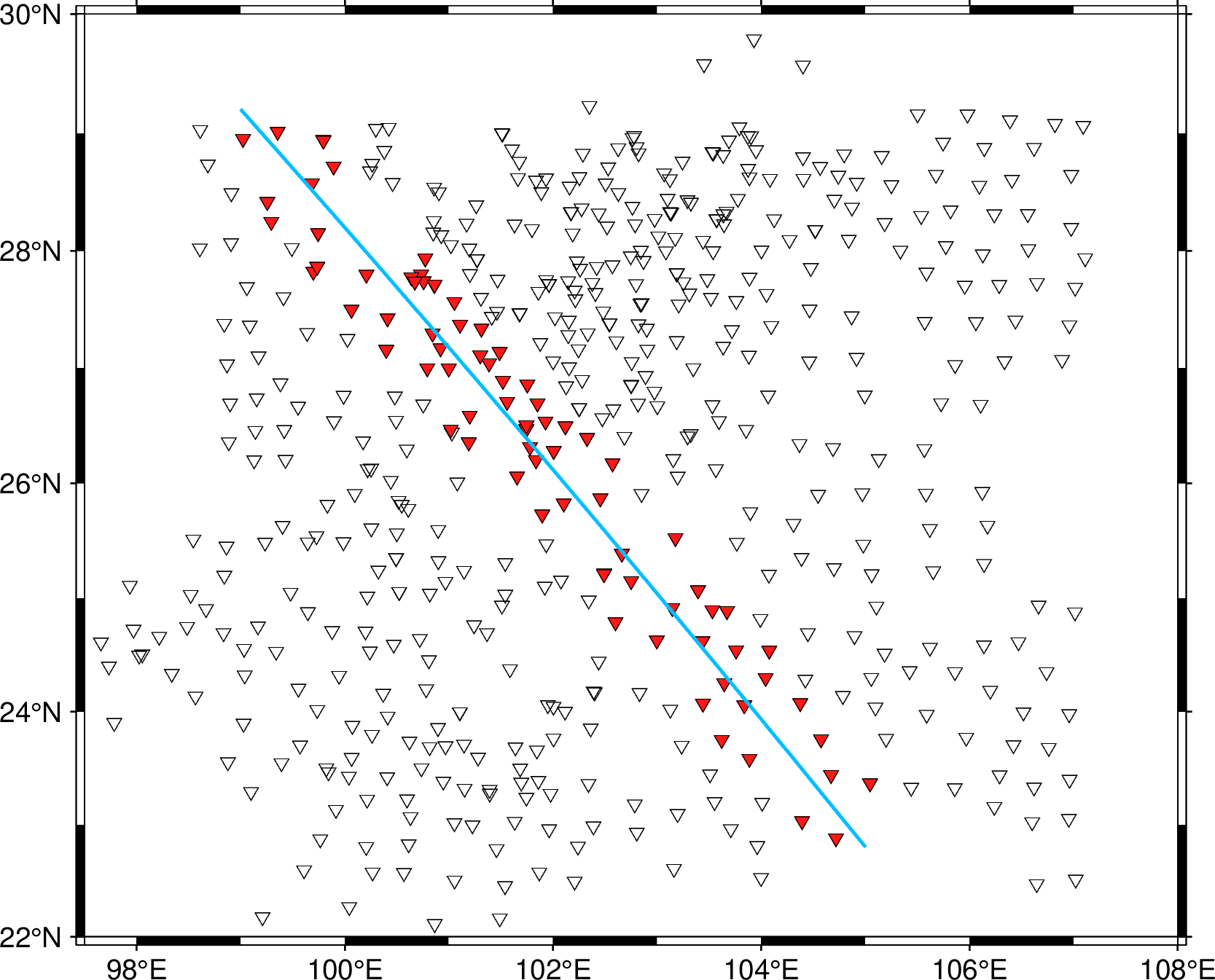
Stations collected from a seismic array. White iverted triangles denote stations in
stalist. Red triangles denote station used for CCP stacking. Blue line denote location of profile.¶Using specified stations: If the
stack_sta_listis set to a existing file, stations in this file are used for CCP stacking. The start and end point of the profile are set in[line]section.Using stations as a linear array with self-adaptive bins: If the CCP stacking is preformed on a curved linear array, a self-adaptive setting of bins maybe suitable. In this case, once
adaptiveis set totrue,slide_valandstack_sta_listis specified, bins are created along the station curve.Note
The
[line]section andrectbins are invalid in such situation.Stations in the
stack_sta_listshould be in order along the linear array
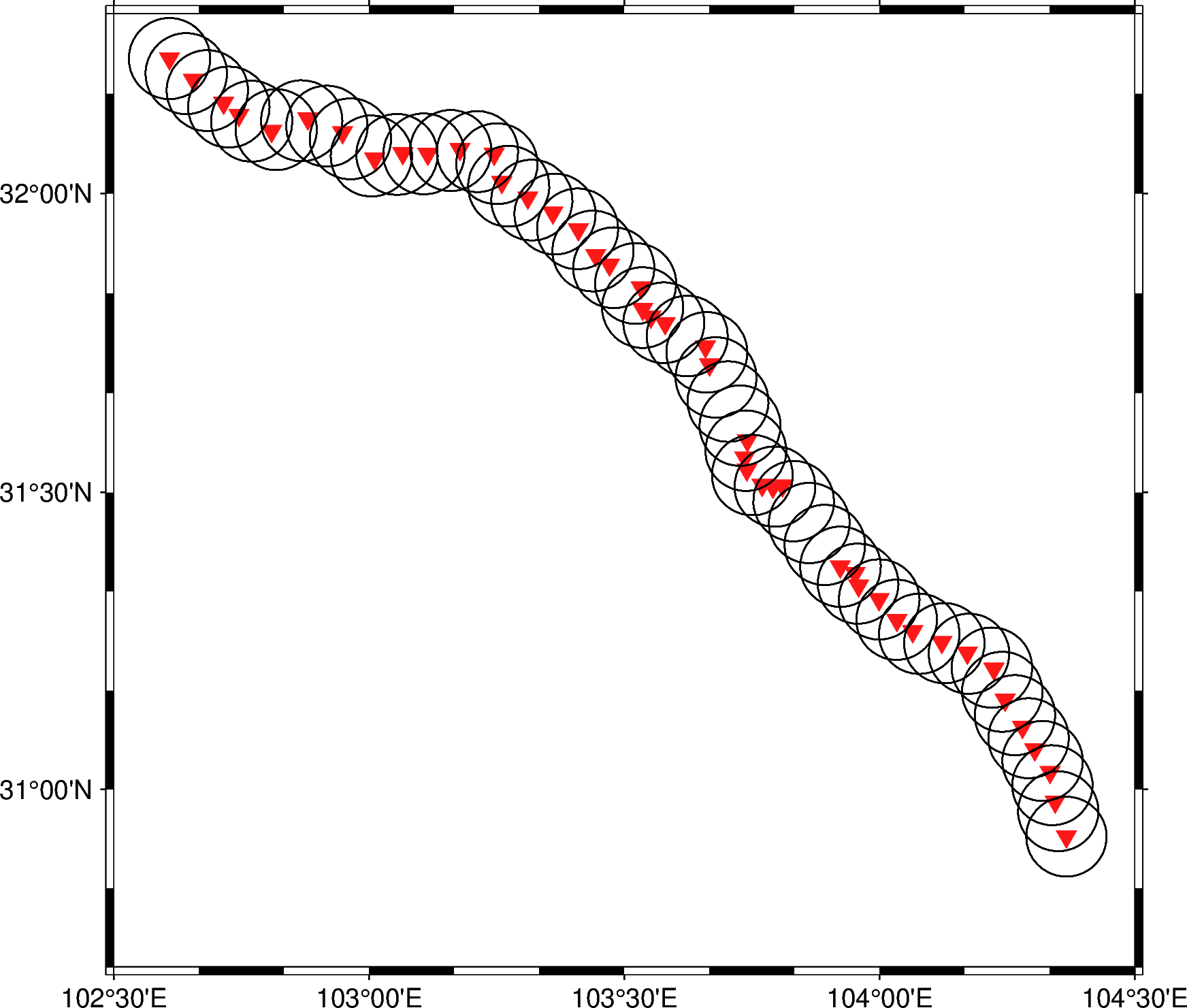
Self-adaptive binning for curved linear array. Red inverted triangles denote stations. Black circles denote location of bins.