Calculate a P-wave Receiver Function (PRF)

Note

• This notebook can be downloaded as PRF_Process.ipynb

• Teleseismic waveforms can be downloaded as rf_example.tar.gz

1. Import corresponding modules

import obspy
import seispy
from seispy.decon import RFTrace
%matplotlib inline

2. Read SAC files with 3 components (ENZ)

You should perpare teleseismic data if SAC format (ENZ) and read them via obspy. To facilitate the follow-up, you’d better write positions of the station and the event into SAC header (i.e., stla, stlo, evla, evlo and evdp).

st = obspy.read('../_static/files/rf_example/*.101.*.SAC')

3. Pre-process for raw data

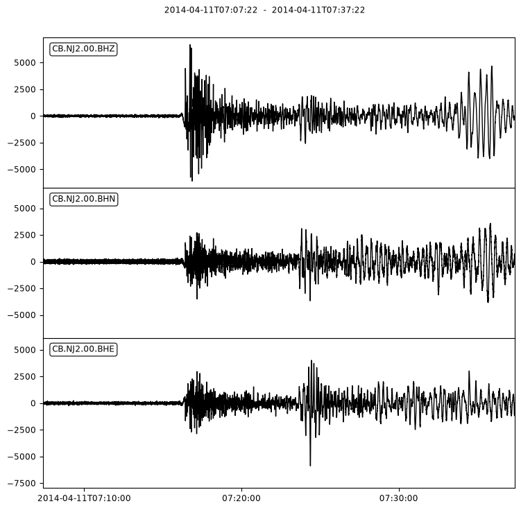
You should remove the mean offset and linear trend of the waveforms, then filtered them with a Butterworth bandpass filter in the range of 0.05–2 Hz. The figures show a comparison between the raw data and the data after pre-process

st.detrend()
st.filter("bandpass", freqmin=0.05, freqmax=2.0, zerophase=True)
st.plot()

4. Calculate the epicenter distance and back-azimuth

To trim the waveform or rotate the components, you can use the seispy.distaz to calculate the epicenter distance and back-azimuth.

da = seispy.distaz(st[0].stats.sac.stla, st[0].stats.sac.stlo, st[0].stats.sac.evla, st[0].stats.sac.evlo)
dis = da.delta
bazi = da.baz
ev_dep = st[0].stats.sac.evdp
print('Distance = %5.2f˚' % dis)
print('back-azimuth = %5.2f˚' % bazi)

Distance = 51.64˚
back-azimuth = 131.59˚

5. Rotation

Now you can rotate horizontal components (ENZ) into radial and transverse components (TRZ)

st_TRZ = st.copy().rotate('NE->RT', back_azimuth=bazi)

6. Estimating P arrival time and ray parameter by obspy.taup

from obspy.taup import TauPyModel

model = TauPyModel(model='iasp91')
arrivals = model.get_travel_times(ev_dep, dis, phase_list=['P'])
P_arr = arrivals[0]

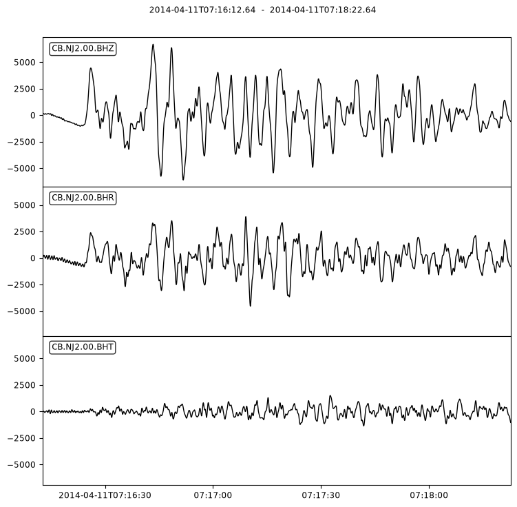
7.Trim the waveforms for PRF

Then you cut 130 s long waveforms around P arrival time (from 10 s before to 120 s after theoretical P arrival times).

dt = st[0].stats.delta
shift = 10
time_after = 120

st_TRZ.trim(st_TRZ[0].stats.starttime+P_arr.time-shift,
            st_TRZ[0].stats.starttime+P_arr.time+time_after)

time_axis = st_TRZ[0].times() - shift
st_TRZ.plot(show=False)

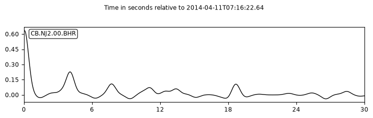
8. Calculate PRF

seispy.decon.RFTrace provide a class for deconvolution. Now let’s Calculate a PRF with iteration time-domain deconvolution mehtod. In this example, we assume:

• Gauss factor = 2.0

• The maximum number of iterations = 400

• Minimum error = 0.001

f0 = 2.0
itmax = 400
minderr = 0.001

rf = RFTrace.deconvolute(st_TRZ[1], st_TRZ[2], method='iter',
                         tshift=shift, f0=f0, itmax=itmax, minderr=minderr)
rf.plot(show=False, type='relative',
        starttime=rf.stats.starttime+shift,
        endtime=rf.stats.starttime+shift+30)